14  lavaan/blavaan + tidySEM

You can combine tidySEM’s layout capabilities with lavaan or blavaan models for visualizations in ggsem. Both frequentist (lavaan) and Bayesian (blavaan) models work seamlessly with this workflow. blavaan objects work identically to how lavaan objects work with tidySEM package in ggsem.

Approach 1: Multi-Group Model with a Shared tidySEM Layout

This method uses tidySEM’s layout specification with multi-group models for consistent visualization across groups.

Use case: Single multi-group model object where ggsem automatically extracts group-specific parameters.

library(lavaan)
library(ggsem)
library(tidySEM)
library(blavaan)

lavaan_string <- 'visual =~ x1 + x2 + x3
             textual =~ x4 + x5 + x6
             speed =~ x7 + x8 + x9'

fit <- sem(lavaan_string, data = HolzingerSwineford1939, group = 'school')
bfit <- bsem(lavaan_string, data = HolzingerSwineford1939, group = 'school')

SAMPLING FOR MODEL 'stanmarg' NOW (CHAIN 1).
Chain 1: 
Chain 1: Gradient evaluation took 0.000564 seconds
Chain 1: 1000 transitions using 10 leapfrog steps per transition would take 5.64 seconds.
Chain 1: Adjust your expectations accordingly!
Chain 1: 
Chain 1: 
Chain 1: Iteration:    1 / 1500 [  0%]  (Warmup)
Chain 1: Iteration:  150 / 1500 [ 10%]  (Warmup)
Chain 1: Iteration:  300 / 1500 [ 20%]  (Warmup)
Chain 1: Iteration:  450 / 1500 [ 30%]  (Warmup)
Chain 1: Iteration:  501 / 1500 [ 33%]  (Sampling)
Chain 1: Iteration:  650 / 1500 [ 43%]  (Sampling)
Chain 1: Iteration:  800 / 1500 [ 53%]  (Sampling)
Chain 1: Iteration:  950 / 1500 [ 63%]  (Sampling)
Chain 1: Iteration: 1100 / 1500 [ 73%]  (Sampling)
Chain 1: Iteration: 1250 / 1500 [ 83%]  (Sampling)
Chain 1: Iteration: 1400 / 1500 [ 93%]  (Sampling)
Chain 1: Iteration: 1500 / 1500 [100%]  (Sampling)
Chain 1: 
Chain 1:  Elapsed Time: 5.259 seconds (Warm-up)
Chain 1:                7.071 seconds (Sampling)
Chain 1:                12.33 seconds (Total)
Chain 1: 

SAMPLING FOR MODEL 'stanmarg' NOW (CHAIN 2).
Chain 2: 
Chain 2: Gradient evaluation took 0.000297 seconds
Chain 2: 1000 transitions using 10 leapfrog steps per transition would take 2.97 seconds.
Chain 2: Adjust your expectations accordingly!
Chain 2: 
Chain 2: 
Chain 2: Iteration:    1 / 1500 [  0%]  (Warmup)
Chain 2: Iteration:  150 / 1500 [ 10%]  (Warmup)
Chain 2: Iteration:  300 / 1500 [ 20%]  (Warmup)
Chain 2: Iteration:  450 / 1500 [ 30%]  (Warmup)
Chain 2: Iteration:  501 / 1500 [ 33%]  (Sampling)
Chain 2: Iteration:  650 / 1500 [ 43%]  (Sampling)
Chain 2: Iteration:  800 / 1500 [ 53%]  (Sampling)
Chain 2: Iteration:  950 / 1500 [ 63%]  (Sampling)
Chain 2: Iteration: 1100 / 1500 [ 73%]  (Sampling)
Chain 2: Iteration: 1250 / 1500 [ 83%]  (Sampling)
Chain 2: Iteration: 1400 / 1500 [ 93%]  (Sampling)
Chain 2: Iteration: 1500 / 1500 [100%]  (Sampling)
Chain 2: 
Chain 2:  Elapsed Time: 4.112 seconds (Warm-up)
Chain 2:                5.879 seconds (Sampling)
Chain 2:                9.991 seconds (Total)
Chain 2: 

SAMPLING FOR MODEL 'stanmarg' NOW (CHAIN 3).
Chain 3: 
Chain 3: Gradient evaluation took 0.000225 seconds
Chain 3: 1000 transitions using 10 leapfrog steps per transition would take 2.25 seconds.
Chain 3: Adjust your expectations accordingly!
Chain 3: 
Chain 3: 
Chain 3: Iteration:    1 / 1500 [  0%]  (Warmup)
Chain 3: Iteration:  150 / 1500 [ 10%]  (Warmup)
Chain 3: Iteration:  300 / 1500 [ 20%]  (Warmup)
Chain 3: Iteration:  450 / 1500 [ 30%]  (Warmup)
Chain 3: Iteration:  501 / 1500 [ 33%]  (Sampling)
Chain 3: Iteration:  650 / 1500 [ 43%]  (Sampling)
Chain 3: Iteration:  800 / 1500 [ 53%]  (Sampling)
Chain 3: Iteration:  950 / 1500 [ 63%]  (Sampling)
Chain 3: Iteration: 1100 / 1500 [ 73%]  (Sampling)
Chain 3: Iteration: 1250 / 1500 [ 83%]  (Sampling)
Chain 3: Iteration: 1400 / 1500 [ 93%]  (Sampling)
Chain 3: Iteration: 1500 / 1500 [100%]  (Sampling)
Chain 3: 
Chain 3:  Elapsed Time: 4.854 seconds (Warm-up)
Chain 3:                7.317 seconds (Sampling)
Chain 3:                12.171 seconds (Total)
Chain 3: 
Computing post-estimation metrics (including lvs if requested)...
lay <- get_layout("visual", "", "","","textual","","speed","", "",
                  "x1", "x2", "x3", "x4", "x5", "x6", "x7", "x8", "x9", rows = 2)

tidysem_object <- prepare_graph(model = fit, layout = lay)
tidysem_object_bayes <- prepare_graph(model = bfit, layout = lay)

plot(tidysem_object)

While tidySEM can plot multiple SEMs at once using a multi-group model object, here we plot them with more aesthetic refinement using ggsem_builder() workflow with the pipe |> operator.

Implementation: You can create structured graph objects from multi-group models using tidySEM’s one layout system.

# Multi-group visualization with positioning (works for both lavaan and blavaan)
ggsem_builder(type = 'sem') |>
  add_group('P', model = fit, object = tidysem_object, y = 25, level = 'Pasteur') |>
  add_group('GW', model = fit, object = tidysem_object, y = -25, level = 'Grant-White') |>
  launch()

# Bayesian version works identically
ggsem_builder(type = 'sem') |>
  add_group('P', model = bfit, object = tidysem_object_bayes, y = 25, level = 'Pasteur') |>
  add_group('GW', model = bfit, object = tidysem_object_bayes, y = -25, level = 'Grant-White') |>
  launch()

Use case: Unified multi-group analysis with consistent visual structure across groups.

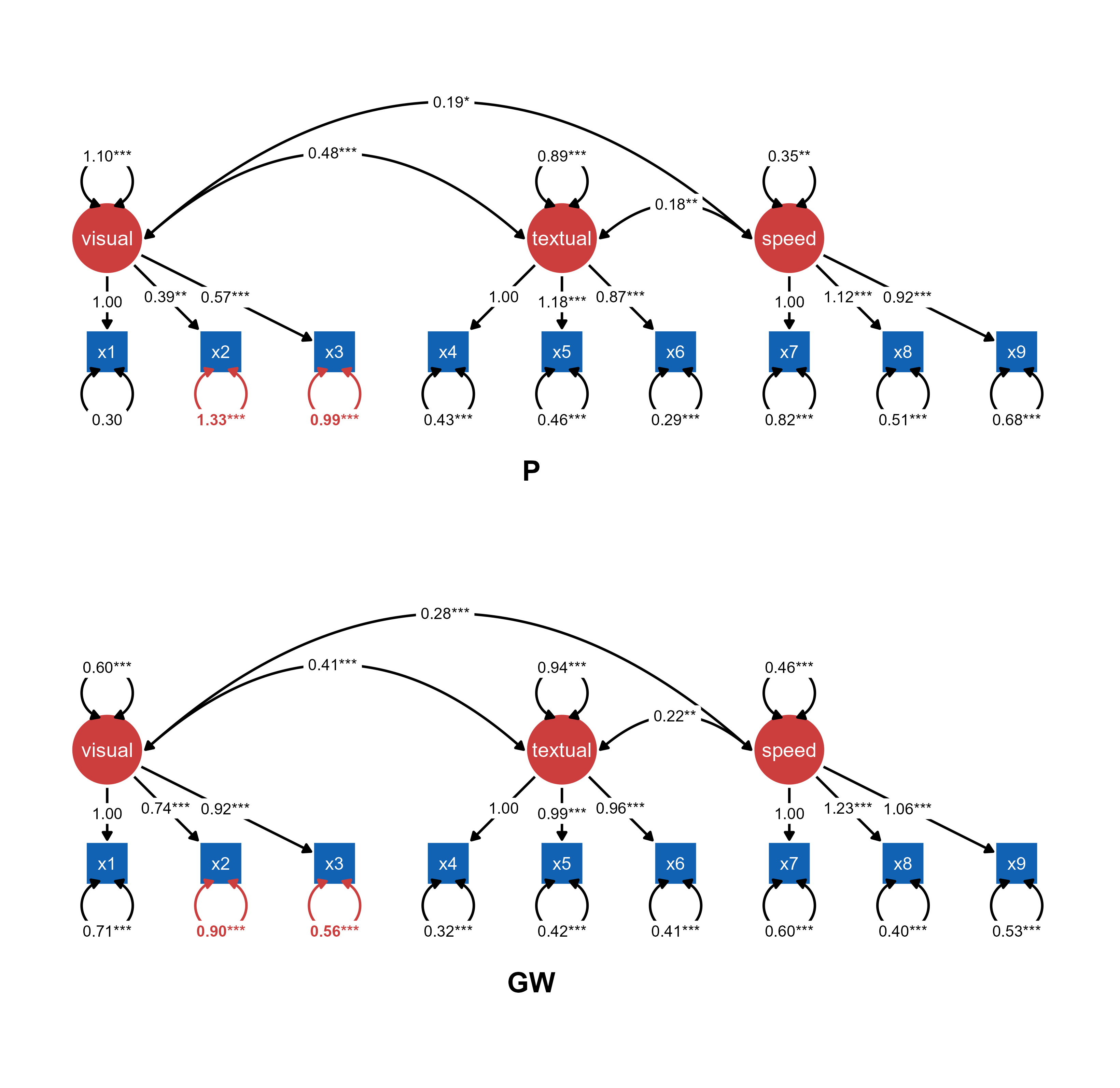
This figure shows a composite multi-group SEM figure (two groups) with significantly different paths highlighted (red color) in ggsem.

Figure 1. A composite multi-group SEM diagram with pre-loaded tidySEM visualization objects and lavaan model objects.

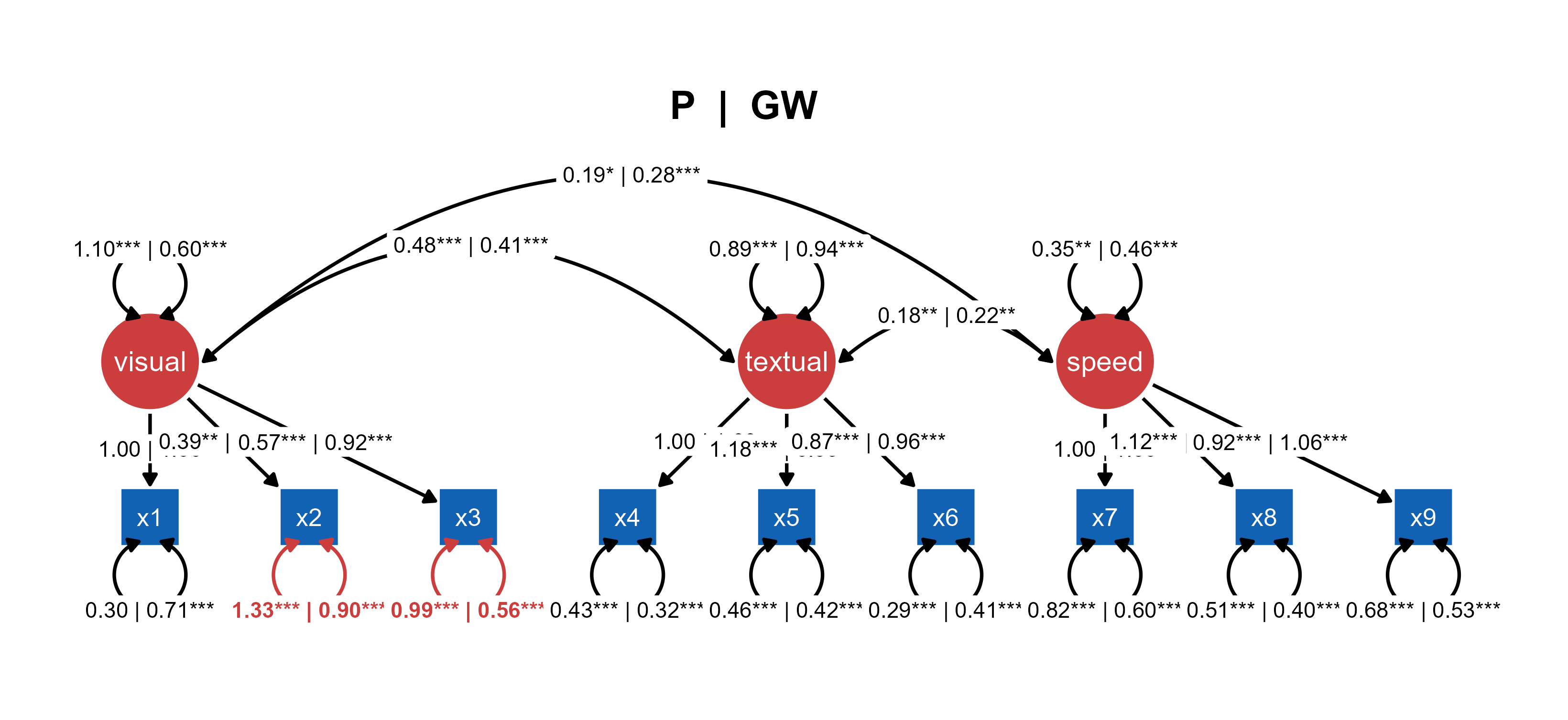
You can also generate a combined SEM of two groups with significantly different paths highlighted (Highlight Group Differences).

Figure 2. A combined multi-group SEM diagram with pre-loaded tidySEM visualization objects and lavaan model objects.

Approach 2: Separate Models with Shared Layout

Fit independent models to subgroup data while maintaining visual consistency through shared layout.

Use case: Pre-rendered diagrams for each group with explicit group-level specification using one model.

# Data preparation
HolzingerSwineford1939P <- HolzingerSwineford1939[HolzingerSwineford1939$school == 'Pasteur',]
HolzingerSwineford1939GW <- HolzingerSwineford1939[HolzingerSwineford1939$school == 'Grant-White',]

# Frequentist models
fitP <- sem(lavaan_string, data = HolzingerSwineford1939P)
fitGW <- sem(lavaan_string, data = HolzingerSwineford1939GW)

tidysem_objectP <- prepare_graph(model = fitP, layout = lay)
tidysem_objectGW <- prepare_graph(model = fitGW, layout = lay)

Visualization: Compare independently fitted models using identical layout structure.

ggsem_builder() |>
  add_group("Ptr", model = fitP, object = tidysem_objectP, y = -20) |>
  add_group("GW", model = fitGW, object = tidysem_objectGW, y = 20) |>
  launch()

Use case: Independent group analyses with standardized visual presentation for direct comparison.

Approach 3: Multi-Group Model with Different tidySEM Layouts

Use a single multi-group model with customized tidySEM layouts for each group to highlight different visual perspectives while maintaining statistical consistency.

Use case: Completely independent models fitted to subgroup data.

# Multi-group model
fit_multi <- sem(lavaan_string, data = HolzingerSwineford1939, group = 'school')

# Custom layouts for each group
lay_pasteur <- get_layout("visual", "", "","","textual","","speed","", "",
                  "x1", "x2", "x3", "x4", "x5", "x6", "x7", "x8", "x9", rows = 2)

lay_grantwhite <- get_layout("", "visual", "","textual","","","","speed", "",
                  "x1", "x2", "x3", "x4", "x5", "x6", "x7", "x8", "x9", rows = 2)

# Prepare group-specific graph objects
graph_pasteur <- prepare_graph(model = fit_multi, layout = lay_pasteur)
graph_grantwhite <- prepare_graph(model = fit_multi, layout = lay_grantwhite)

Implementation: Apply distinct visual organizations to the same multi-group model for comparative analysis.
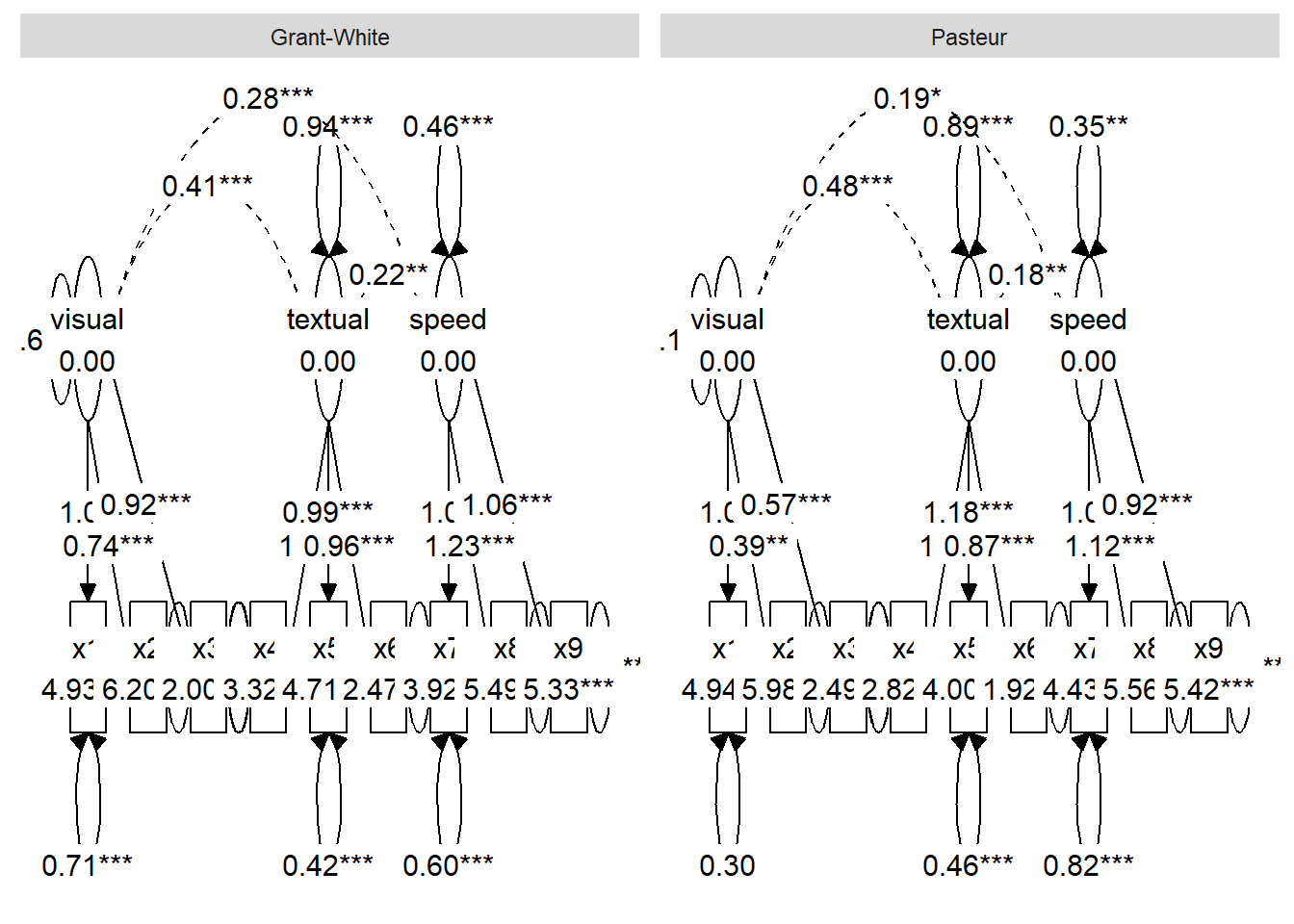
ggsem_builder(type = 'sem') |>
  add_group('Pasteur', model = fit_multi, object = graph_pasteur, y = 20, level = 'Pasteur') |>
  add_group('Grant-White', model = fit_multi, object = graph_grantwhite, y = -20, level = 'Grant-White') |>
  launch()

Use case: Comparative visualization of multi-group results using customized layouts that emphasize different aspects of the model structure for each group, while maintaining statistical consistency through shared parameter estimation.

Key Note: All three approaches work identically with both lavaan and blavaan models. Simply replace sem() with bsem() and the visualization workflow remains unchanged.