Instead of beginning with an empty workspace in ggsem(), you can load Bayesian structural equation modeling objects and associated visualizations to initialize the application with pre-existing content. There are three primary strategies for handling multiple groups using Bayesian estimation:
Note: The first click of Apply Changes button for each group might be quite slow (or when you change layout or statistical annotations of the SEM diagram). This is because when the click is trigger, the app organizes all the metadata, and Bayesian SEM model (blavaan) is computationally heavy. See at the end of the chapter for an alternative solution.
Approach 1: Single Multi-Group Model
This approach leverages blavaan’s integrated multi-group capability, particularly suitable for Bayesian measurement invariance analysis.
Use case: A multi-group Bayesian model where ggsem retrieves group-specific parameter distributions.
Model Description: A single multi-group Bayesian SEM object that estimates the three-factor confirmatory factor analysis separately for each school.
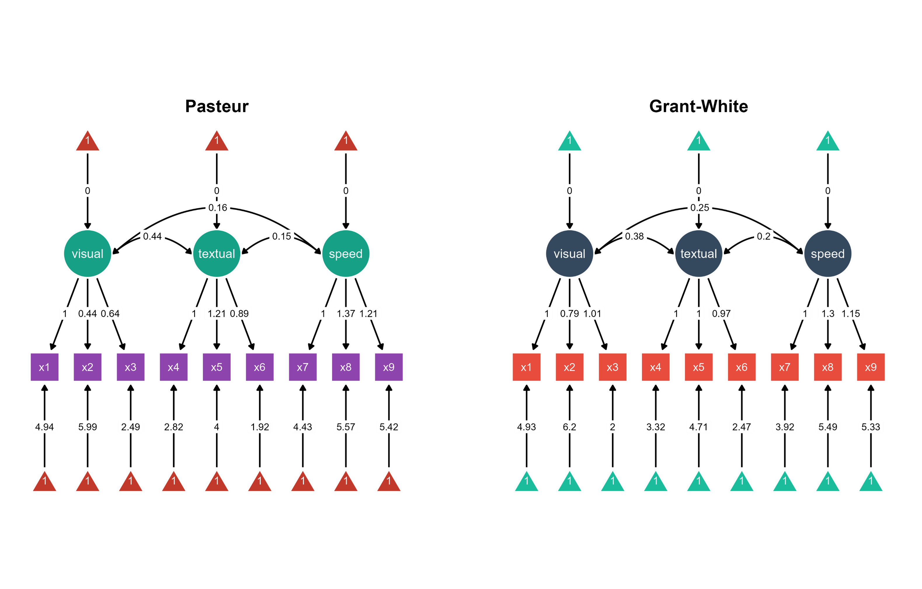
ggsem_builder() |>add_group(name ="Pasteur", object = bfit, x =-35) |>add_group(name ="Grant-White", object = bfit, x =35) |>launch()
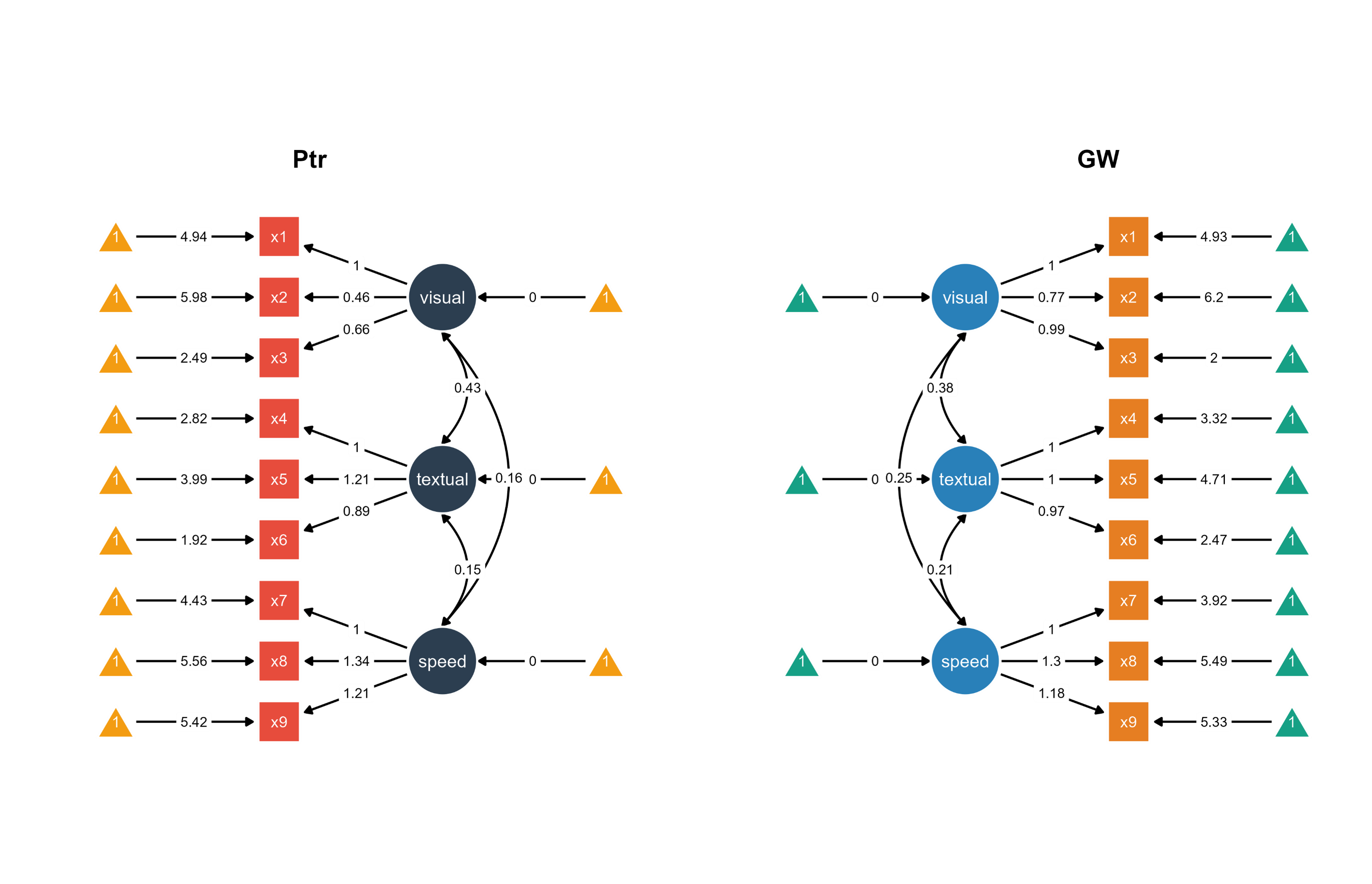
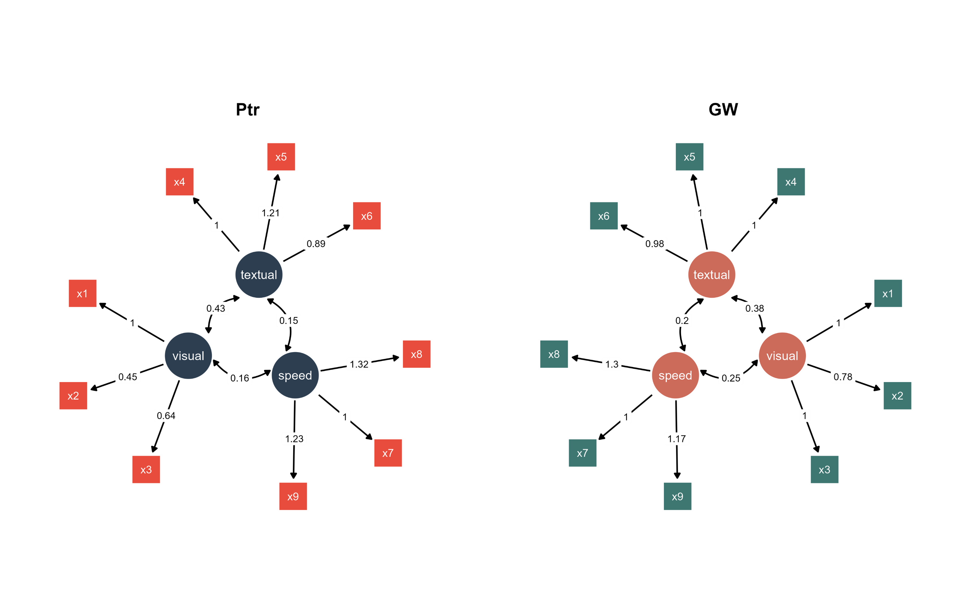
Figure 1. Two Bayesian SEM diagrams side-by-side with unique color palettes.
Visualization: ggsem extracts group-specific Bayesian parameter estimates from the multi-group model, arranging the Pasteur school visualization on the left (x = -35) and Grant-White on the right (x = 35).
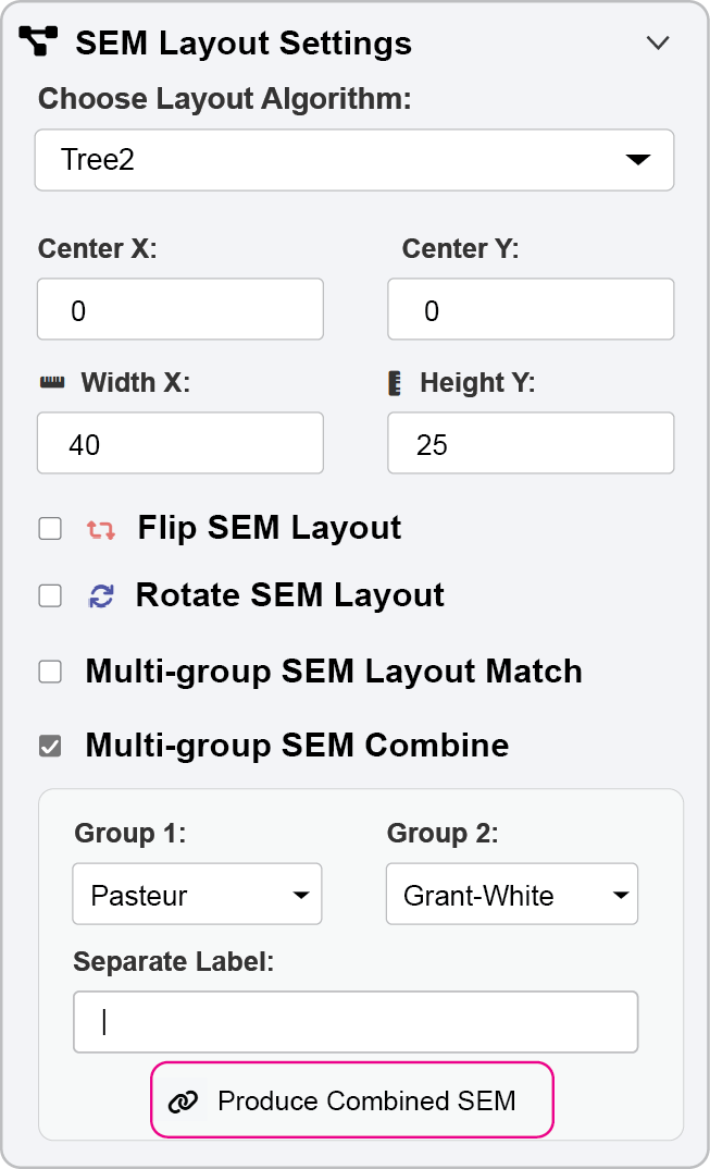
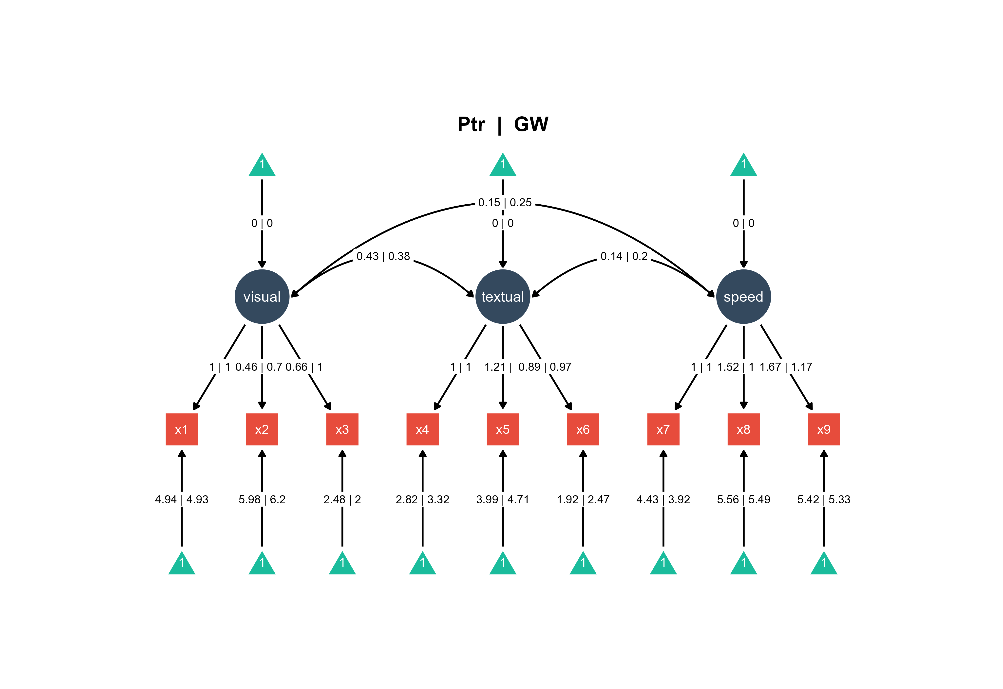
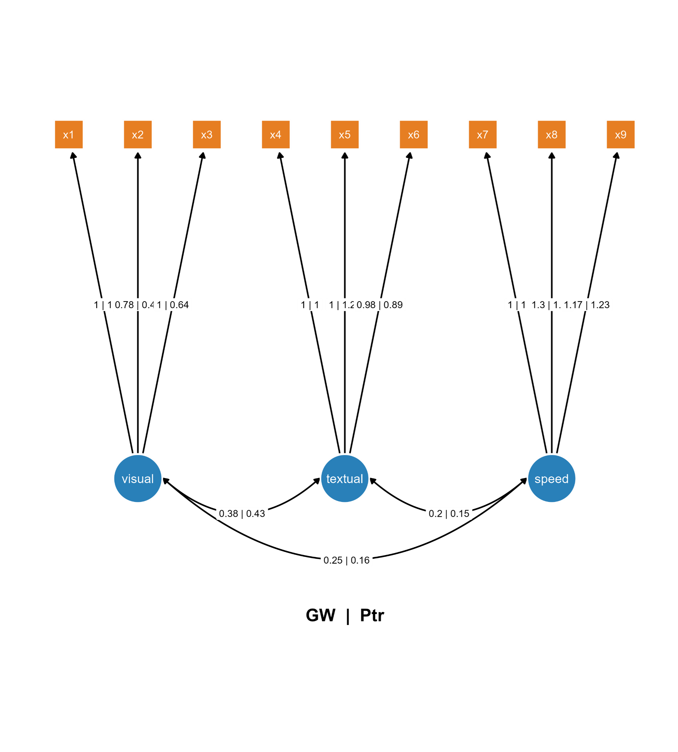
You can also combine the two SEMs into one SEM diagram.
Figure 2. Combine the two Bayesian SEMs across groups into one diagram
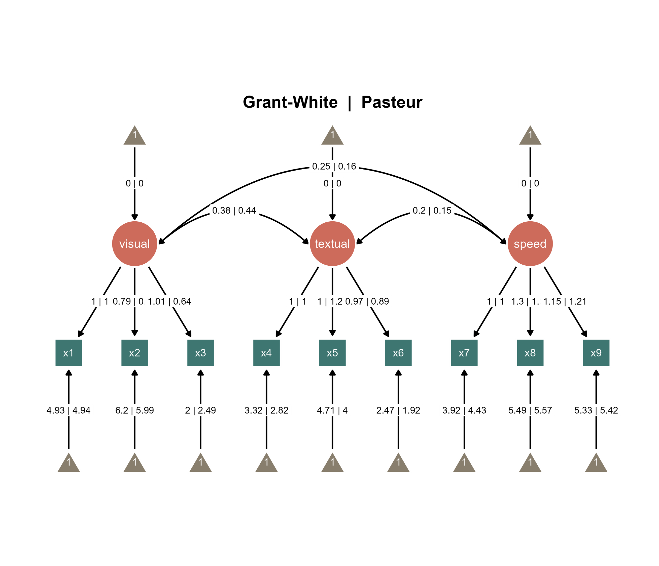
If you add the title automatically using options in Aesthetic Grouping (see Chapter 16), this is the output:
Figure 3. A combined Bayesian SEM diagrams with automatically generated title.
Using interactive parameter visualization, you can modify the angle of one node group in the Latent Group Orientation submenu. The orientations of visual and speed node groups (with their associated intercept and observed nodes) have been modified.
Figure 4. A combined SEM diagrams with automatically generated title and modified layout using interactive parameter visualization.
Approach 2: A Multi-Group Model with Pre-configured Visualizations
This methodology combines the analytical advantages of a multi-group Bayesian framework with customized graphical representations from semPlot.
Use case: Pre-generated diagrams for individual groups utilizing a single Bayesian model with group-specific display parameters.
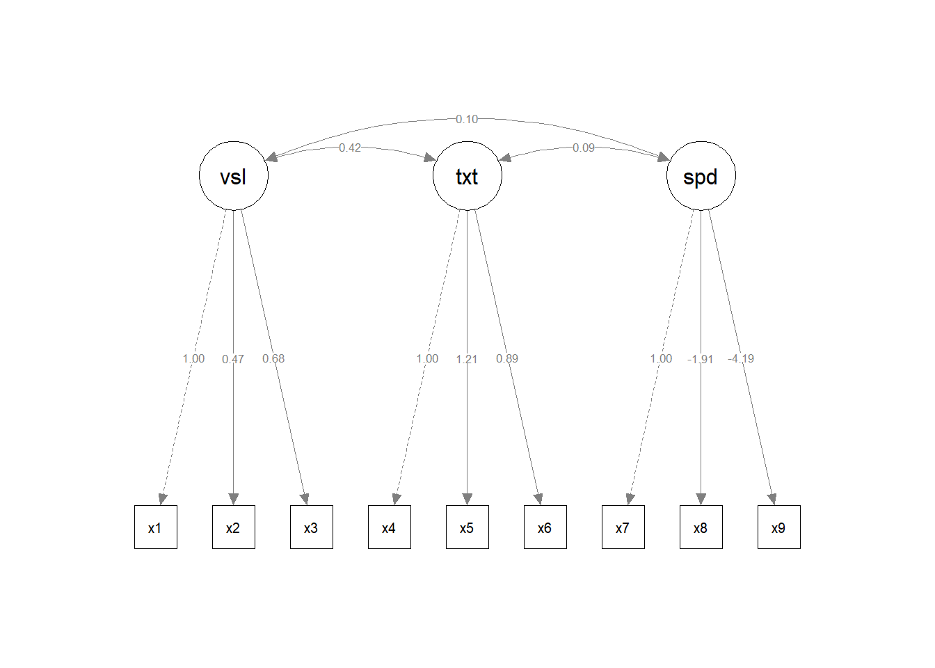
plot.new() # to prevent error, reset the plotting spacesem_paths <-semPaths(bfit, layout ="tree2",what ="paths",intercepts =TRUE,whatLabels ="est",style ="lisrel",residuals =FALSE)
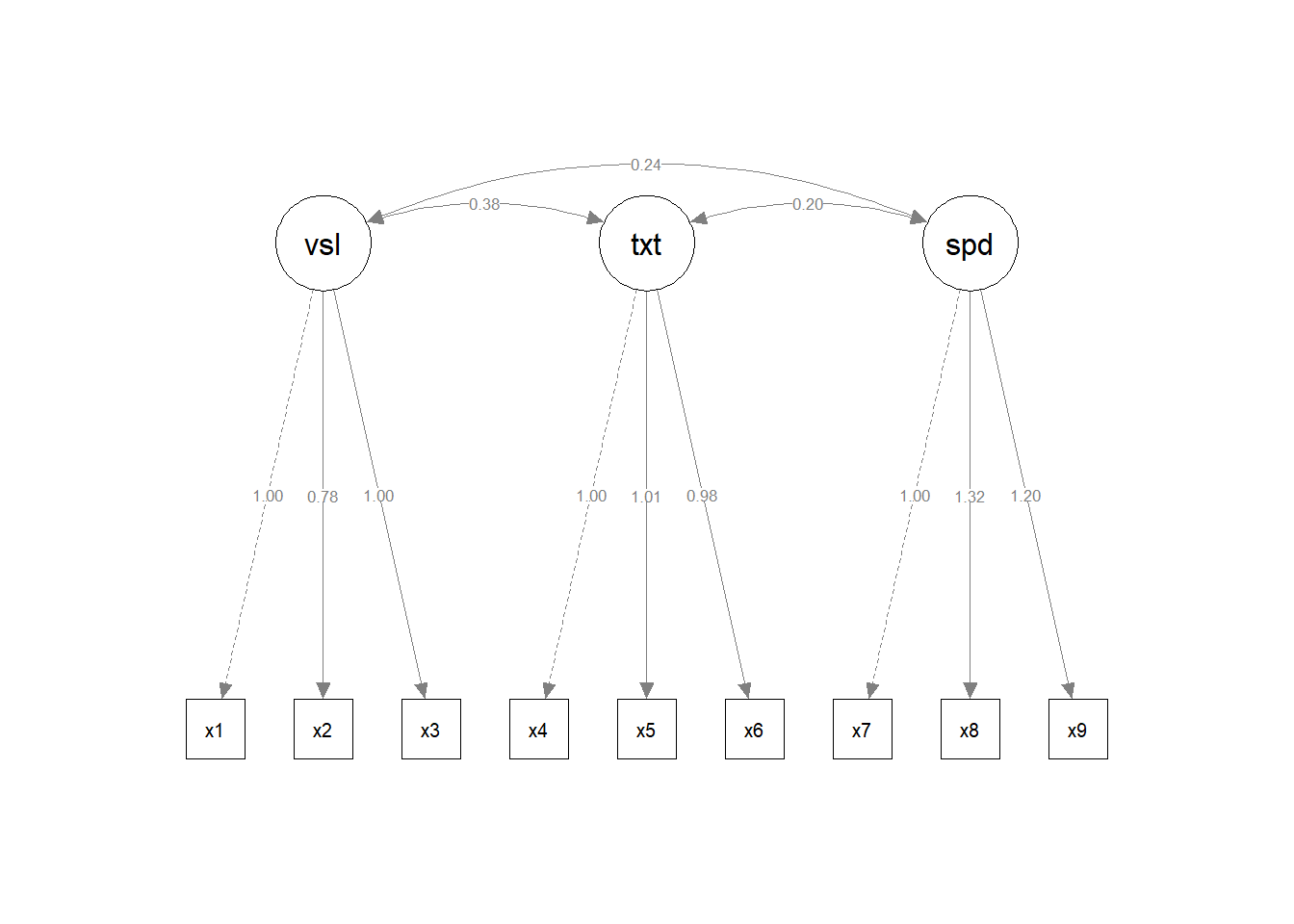
Visualizations: The multi-group semPaths output is split into two separate plot objects (sem_paths1 and sem_paths2), each containing the pre-rendered diagram for one school group with parameter estimates displayed.
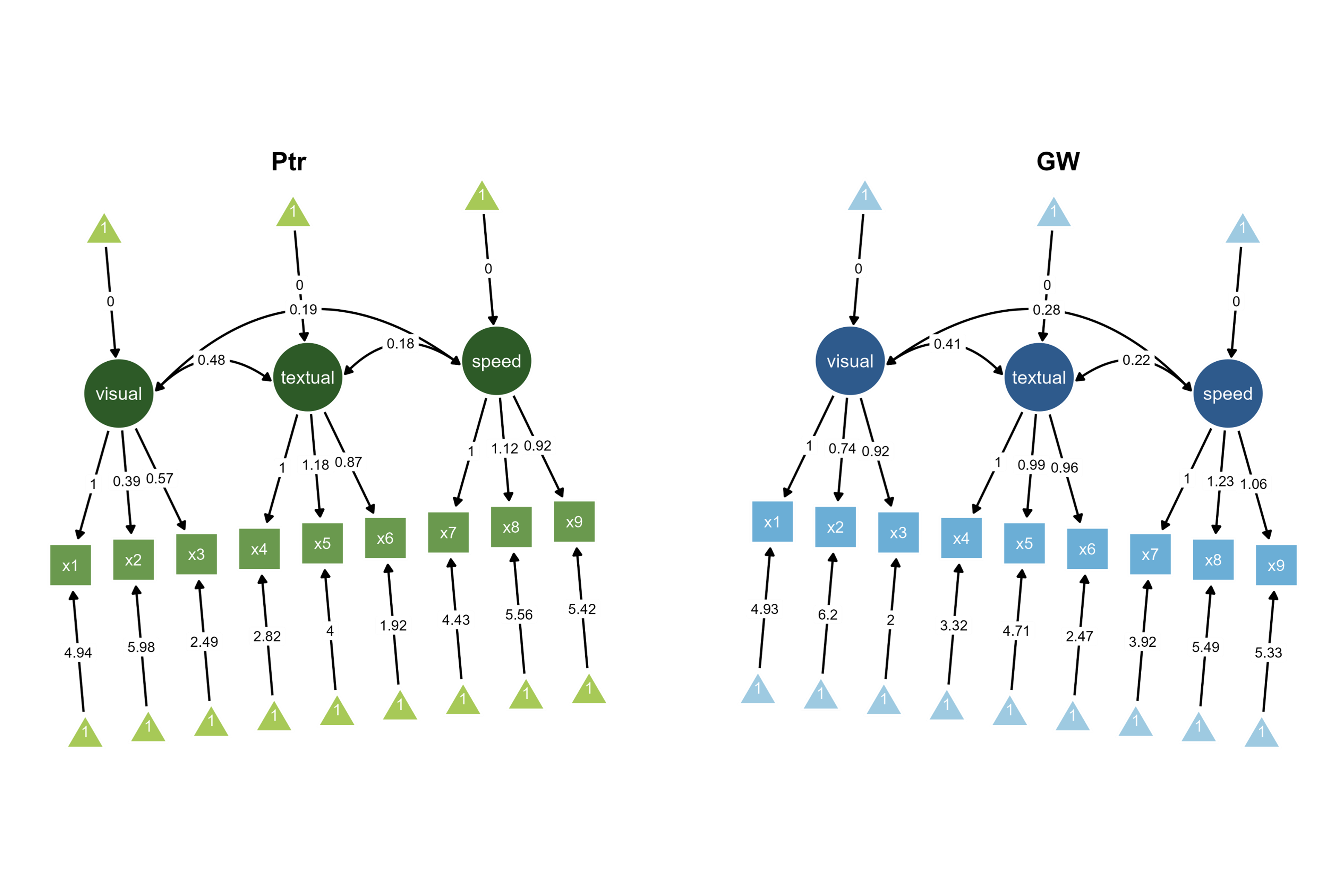
ggsem_builder() |>add_group("Ptr", model = bfit, object = sem_paths1, x =-35, level ="Pasteur") |>add_group("GW", model = bfit, object = sem_paths2, x =35, level ="Grant-White") |>launch()
Figure 5. Two Bayesian SEM diagrams side-by-side with unique color palettes with different orientations (+/- 90 degrees).
First, the layout of the second SEM group was flipped horizontally. Then, the orientation was modified for each group using options in the SEM Layout submenu (+/- 90 degrees).
Integration: Use the same multi-group Bayesian model object but with pre-loaded visualizations. The level parameter directly maps each diagram to its corresponding group in the model, so level has to match each group name in the original data file.
With this approach, you can also combine the two SEMs as shown in Figure 2.
Figure 6. A combined Bayesian SEM diagrams with automatically generated title.
Approach 3: Independent Single-Group Models
This strategy approaches each group as entirely separate entities, applying distinct Bayesian models to partitioned datasets.
Use case: Fully autonomous Bayesian models applied to subgroup data with independent estimation procedures.
Analysis Workflow: The dataset is split into school-specific subsets, then identical three-factor CFA models are fitted independently to each school’s data, creating separate model and visualization objects with school-specific posterior distributions.
ggsem_builder() |>add_group("Ptr", model = bfitP, object = sem_pathsP, x =-35) |>add_group("GW", model = bfitGW, object = sem_pathsGW, x =35) |>launch()
Figure 7. Two Bayesian SEM diagrams side-by-side. One of them has a flipped layout.
Comparison: The interactive application positions the independently fitted Pasteur and Grant-White models side-by-side, allowing visual comparison of parameter estimates that were calculated separately for each school without multi-group constraints.
With this approach, you can also combine the two SEMs as shown in Figure 2. However, you cannot create combined SEM with one frequentist model (sem() from lavaan) and one Bayesian model (bsem() from blavaan).
Figure 8. A combined SEM with vertically flipped layout and automatically generated title at bottom center.
Note: blavaan object is computationally heavy, and it works slowly with semPlot function. Alternatively, try with tidySEM instead (next chapter).