library(ggsem)
ggsem()2 App Overview
The ggsem package empowers users to dynamically interact with parameters in diagrams display relational data. The core of the package is its locally-run Shiny application, which can be launched with the code below:
2.1 Overview of the ggsem App Interface
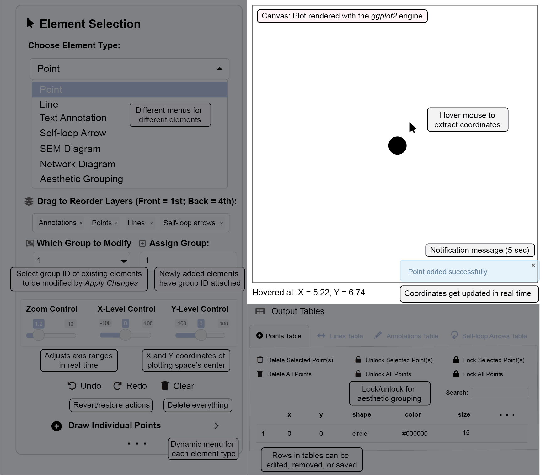
The ggsem application provides an interactive environment for creating and customizing network diagrams and Structural Equation Modeling (SEM) visualizations (Figure 1). The interface is logically divided into two main sections: the plotting canvas on the right and the control sidebar on the left.
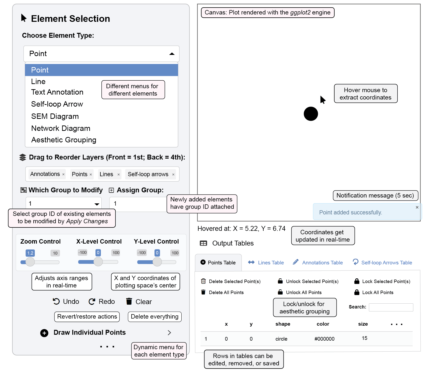
ggsem App interface2.2 The Plotting Canvas
This is the primary workspace where your diagrams are rendered in real-time (Figure 2). As you add elements and adjust settings in the sidebar, the visualization here updates interactively.
2.3 The Control Sidebar
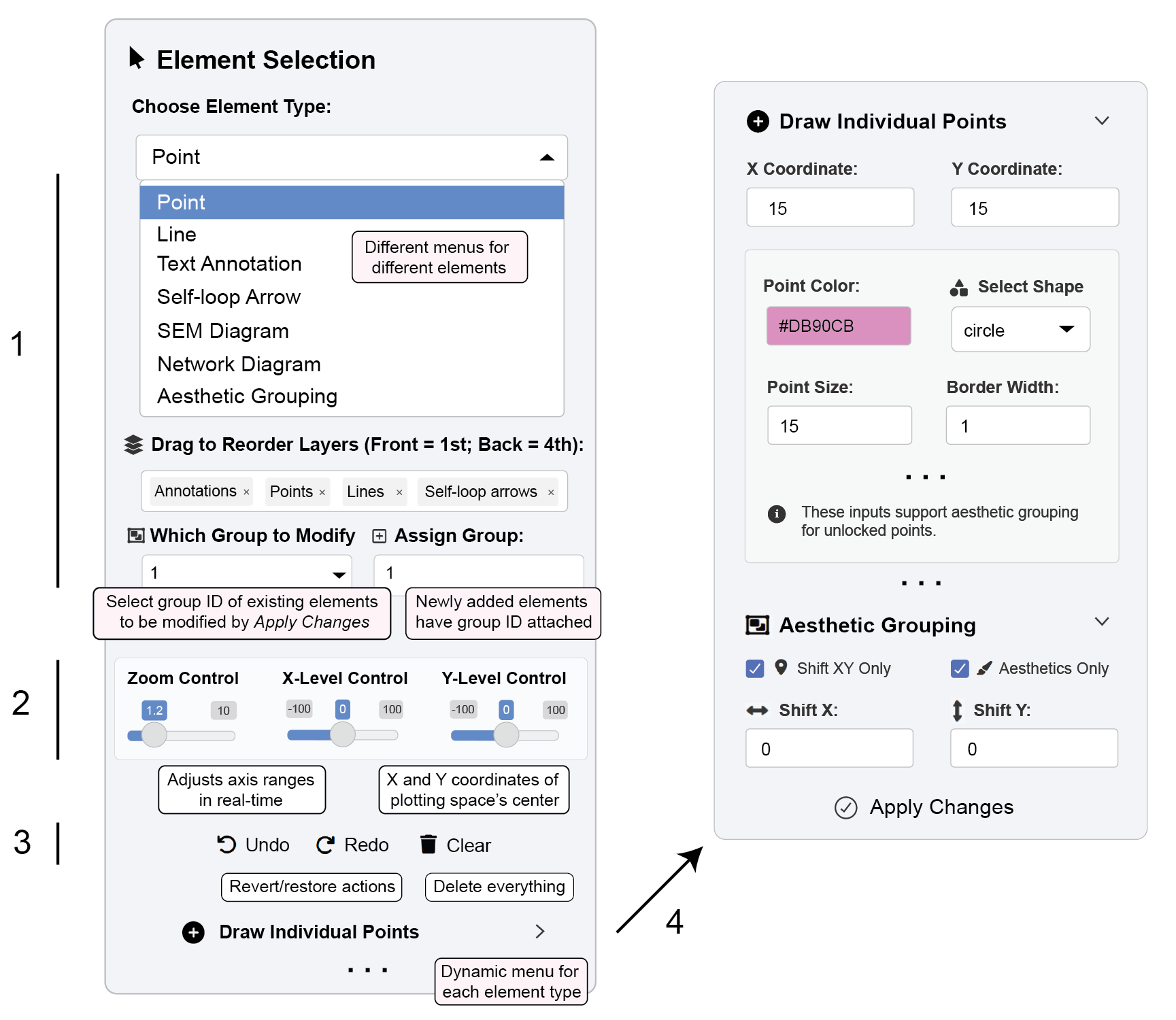
The left sidebar (Figure 3) contains all the tools for building and customizing your diagram. It is organized into several key areas:
- Element Selection & Management
Element Type: This dropdown menu is the starting point for all creation. It allows you to select the type of element you wish to add or modify. The options are:
Point: For adding individual nodes.
Line: For drawing edges, connectors, or arrows between points.
Text Annotation: For adding labels or mathematical expressions.
Self-loop Arrow: For creating circular arrows that connect a node to itself.
SEM Diagram: A specialized section for generating path diagrams from
lavaanmodel syntax, with optional AI-assisted model generation.Network Diagram: For creating network visualizations directly from edge list or adjacency matrix CSV files.
Aesthetic Grouping: For applying bulk changes to the appearance and position of multiple elements at once.
Layer Ordering: This feature controls the visual stacking order (z-index) of the elements on the canvas. You can drag the layers (Annotations, Points, Lines, Self-loop arrows) to reorder them. The top item in the list will appear in the front, potentially obscuring elements in layers below it. The default order ensures points are displayed on top of lines.
Group Assignment: When adding new elements, you can assign them to a specific aesthetic group. This feature allows you to later modify all elements within that group simultaneously (e.g., change the color of all points in “Group 1”).
- Viewport Controls
These controls adjust your view of the canvas without altering the underlying data.
Zoom Control: A slider and numeric input to zoom the canvas in and out (from 0.1x to 10x de-magnification).
X-Level & Y-Level Control: Sliders and numeric inputs to pan the canvas horizontally and vertically. This is essential for navigating diagrams that extend beyond the initial viewport.
- Action History & Canvas Management
Undo/Redo Buttons: Revert or reapply your recent actions. These are also accessible via standard keyboard shortcuts (
Ctrl+ZandCtrl+Y). The app maintains a full history of your session.Clear Button: Removes all elements from the canvas to start a new diagram.
- Dynamic Element-Specific Panels
This is the most dynamic area of the sidebar. Its content changes contextually based on your selection in the Element Type dropdown, and remembers settins for each Group in Which Group to Modify dropdown. Each panel provides detailed controls for the chosen element:
For Points: Options to draw individual points, automatically arrange unlocked points into layouts (circle, grid, star, etc.), apply color gradients, lock points to prevent modification, and perform bulk aesthetic shifts.
For Lines: Controls for manually drawing straight or curved lines/arrows, auto-generating edges between unlocked points based on connection rules (e.g., fully connected, nearest neighbor), applying gradients, and bulk editing.
For Text Annotations: Tools for adding single text labels or math expressions, auto-generating labels on unlocked points (as numbers, letters, or custom text), and managing text aesthetics in groups.
For Self-loop Arrows: Inputs for creating individual loops or auto-generating them on unlocked points, with controls for radius, gap size, orientation, and gradient effects.
For SEM Diagrams: A comprehensive suite of tools including:
Data & Model Input: Upload a CSV dataset and define your model using
lavaansyntax, with an innovative AI assistant to help generate the syntax from your data structure or a natural language description.Layout & Statistics: Choose from various SEM-specific layouts and display model fit indices.
Interactive Customization: Fine-tune the appearance and positions of individual nodes, edges, and labels, or modify them in groups.
For Network Diagrams: Functionality to upload network data (CSV), select a layout algorithm, and extensively customize the aesthetics of nodes, edges, and labels, including edge curvature and scaling width by weight.
For Aesthetic Grouping: A centralized panel for managing elements by their group labels. You can shift positions, change aesthetics, rename groups, show/hide group labels, align groups, or delete/lock all elements within a specific group.
2.3.1 Real-time Data Tables
As you add graphical elements to the canvas, four interactive data tables are automatically updated in the Output Tables section:
Points Table - Records all nodes with their coordinates, colors, sizes, shapes, and group assignments
Lines Table - Contains all edges with start/end coordinates, line types, colors, widths, and arrow specifications
Annotations Table - Stores text labels with positioning, font properties, colors, and mathematical expressions
Self-loop Arrows Table - Tracks circular arrows with center points, radii, gap sizes, and orientation angles
Key features of the data tables:
Direct Editing: Click on any cell to modify values directly (X/Y coordinates, colors, sizes, etc.)
Bulk Operations: Use the action buttons above each table to delete, lock, or unlock selected or all elements
Visual Feedback: Changes made in the tables instantly update the visualization
Group Management: See and manage the group assignments for all elements
2.4 Quick Workflow Example
While the most powerful feature of ggsem is its ability to create and customize Structural Equation Models, I present a typical workflow to generate graphical elements such as points and lines.
2.4.1 Part 1: Draw Points
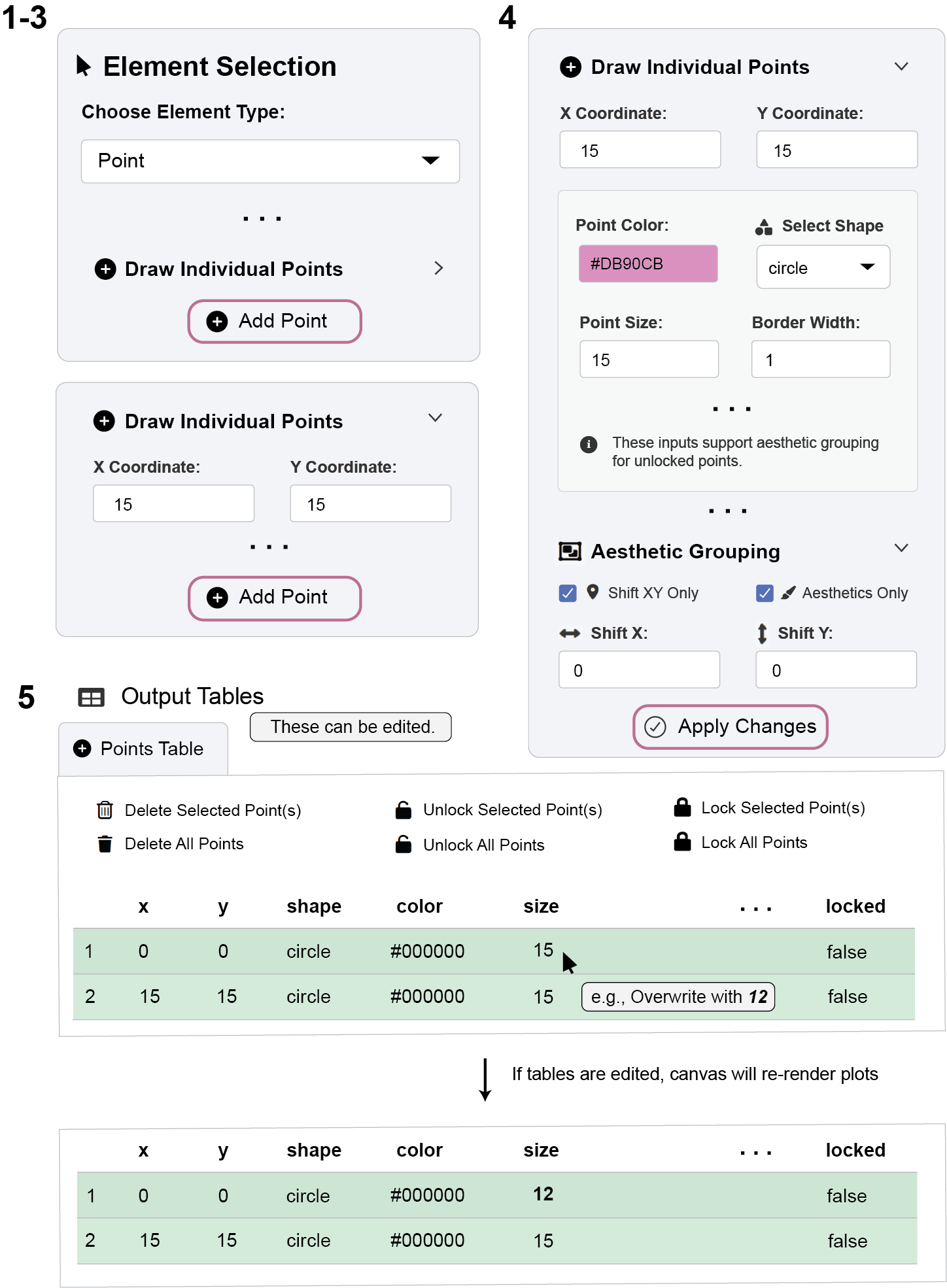
- Choose an Element Type from the dropdown (e.g., Point).
- Use the options in the Sidebar to add elements to the canvas (e.g., click “Add Point”).
Click Add Point without changing any settings. This creates a black point at the origin (x = 0, y = 0).
Create another point. But change the settings so that its coordinate is at x = 15, y = 15, and modify its color setting.
- Use the Viewport Controls to zoom and pan for a better view.
- Try modifying the aesthetics (points) of existing elements by clicking Apply Changes.
Any changes done via Apply Changes will be applied to unlocked points.
Try to Lock points to see what happens.
- Use Undo/Redo freely to experiment, as well as directly edit information in the Output Tables. Any changes will update the plotting canvas in real-time.
2.4.2 Part 2: Connect the Points with a Line
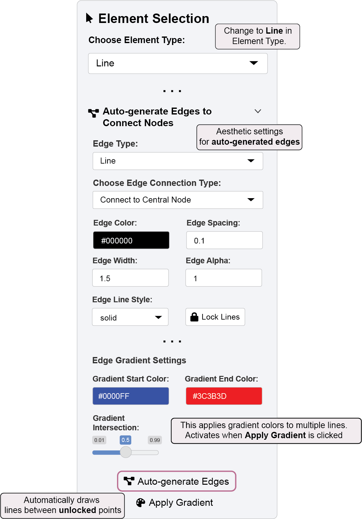
- Switch the Element Type (e.g., to Line) to connect your points, either manually or using the “Auto-generate Edges” button.
Edges are formed only between unlocked points.
Undo your actions and experiment with the locking mechanism. Try to Lock points and see if edges can be formed automatically using “Auto-generate Edges” button.
Note: Rows are green if they are unlocked. They become red if they are locked.
2.4.3 Part 3: Label Points with Texts
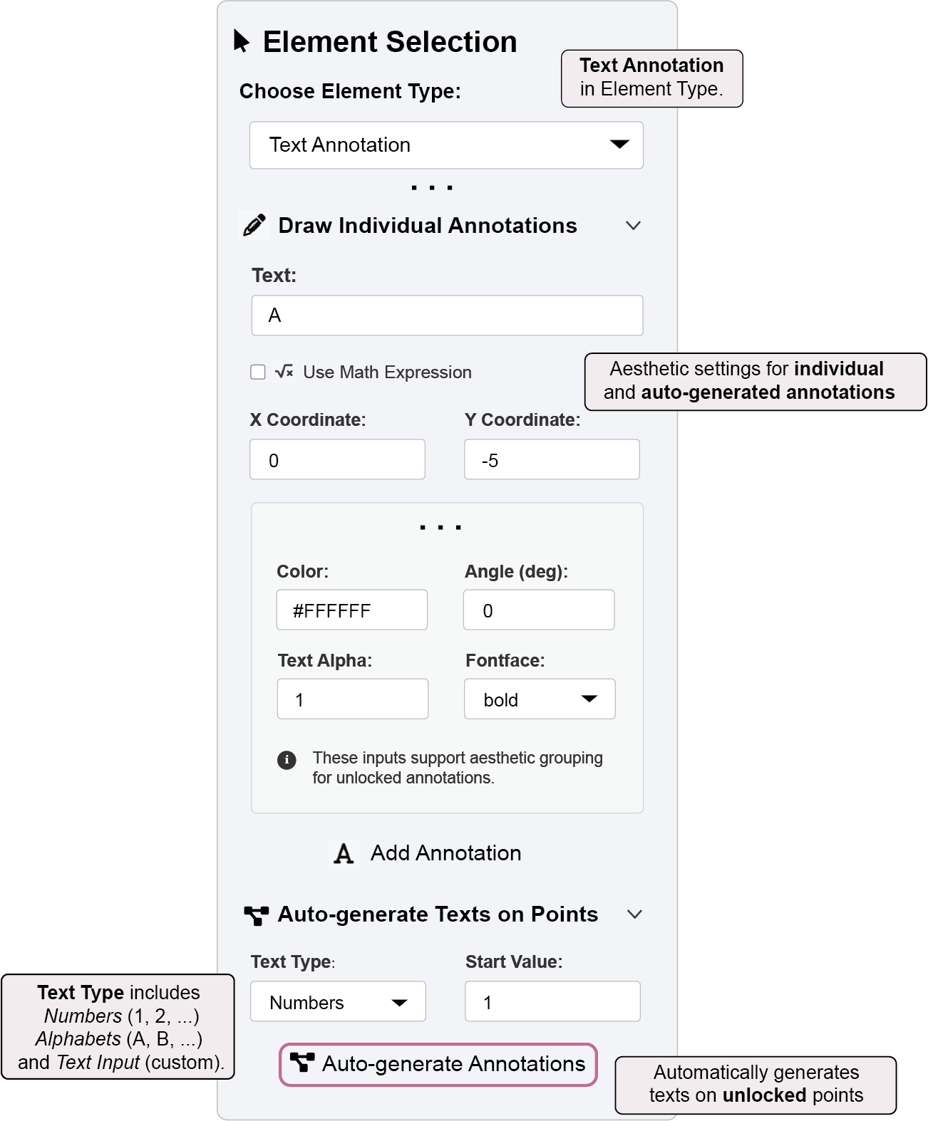
- Switch the Element Type (to Annotation) to label your points automatically using the “Auto-generate Annotations” button.
Aesthetics options can be accessed in Draw Individual Annotations sub-menu.
Make the labels visible by choosing a white (#FFFFFF) or similar color.
2.5 Export & Import CSV Files
Saving Your Work:
- Use the “Choose CSV to Download” dropdown to select which element type to export
- Click “Download Selected CSV” to save individual element tables
- These CSV files contain all the aesthetic properties needed to recreate your visualization
Resuming Your Work:
You can continue to work across multiple sessions or share visualizations with collaborators.
- Use the file inputs to upload previously saved CSV files
- Load Points CSV, Lines CSV, Annotations CSV, and Self-loop Arrows CSV to restore your entire diagram
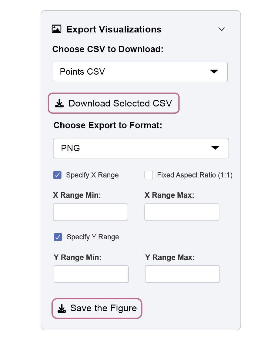
2.6 Figure Export Options
ggsem allows you to download your diagrams in multiple formats:
PNG & JPEG - For presentations and web use
PDF & SVG - For publication-quality vector graphics
Custom Export Settings:
Fixed Aspect Ratio (unchecked by default) - Maintains 1:1 proportions
Specify X/Y Range - Define custom viewport dimensions for asymmetric figures
Range Inputs - Set minimum and maximum values for precise cropping
For your diagram, you can:
- Double-check if the Fixed Aspect Ratio box is unchecked.
- Do not provide any specific x or y ranges (Figure 6). Then the app will automatically determine the appropriate range.
- Save the image in PNG file.
2.7 Recreate Your Figure by Code
R-savvy users might want to access the figure in code form to freely decompose and modify each component. This is possible because ggsem relies on ggplot2 framework to render plots using these steps and CSV outputs from the app:
library(ggsem)Documentation website of ggsem: smin95.github.io/ggsem/points <- read.csv('app_overview/points.csv')
lines <- read.csv('app_overview/lines.csv')
annotations <- read.csv('app_overview/annotations.csv')
ggsem_data <- list(points, lines, annotations) # Put them in a list, any order is fineLoad
ggsemlibrary into memory.Load the CSV files from your directory and save them into objects
pointscan store thepoints.csvfilelinescan store thelines.csvfileannotationscan store theannotations.csvfile
Create a list with the three objects stored (e.g.,
ggsem_data).Use
csv_to_ggplot()to convert the CSVs intoggplotobject (see below). Axis ranges are automatically determined similarly to how theggsemapp sets for saving image outputs.
plot1 <- csv_to_ggplot(ggsem_data)Coordinate system already present. Adding new coordinate system, which will
replace the existing one.- Save the image using
save_figure()from theggsempackage.This function has no input for width or height because the figure ratio can be disrupted if they are manually chosen (due to how
ggplot2stores graphics).save_figure()automatically determines the appropriate width and height.
save_figure('plot1.png', csv_to_ggplot(ggsem_data))
2.7.1 Modify the graphics outside the app
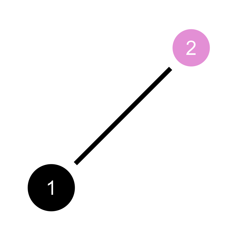
You can directly modify the width of the edge connecting the points at the level of the data frame lines.
lines x_start y_start x_end y_end ctrl_x ctrl_y ctrl_x2 ctrl_y2
1 2.58211 2.58211 12.79289 12.79289 NA NA NA NA
curvature_magnitude curvature_asymmetry rotate_curvature type
1 0 0 FALSE Straight Line
color end_color color_type gradient_position width alpha arrow arrow_type
1 #000000 NA Single NA 1 1 NA NA
arrow_size two_way lavaan network line_style locked group
1 NA NA FALSE FALSE solid FALSE 1The width of the line is set to 1, which we can increase to 2.
lines$width <- 2Now, as before, convert the updated CSV files to ggplot object again using csv_to_ggplot(), and save the object into an image file using save_figure().
ggsem_data <- list(points, lines, annotations) # Put them in a list, any order is fine

plot2 <- csv_to_ggplot(ggsem_data)
Coordinate system already present. Adding new coordinate system, which will
replace the existing one.save_figure('plot2.png', plot2)